
Table of Contents
Bayesian optimization with adaptive kernels for robot control
Ruben Martinez-Cantin, “Bayesian optimization with adaptive kernels for robot control”, 2017 IEEE International Conference on Robotics and Automation (ICRA), 2017, pp. 3350–3356.
I. INTRODUCTION
In this paper, we present a kernel function specially designed for Bayesian optimization, that allows nonstationary modeling without prior knowledge, using an adaptive local region. The new kernel results in an improved local search (exploitation), without penalizing the global search (exploration),
Earliest versions of Bayesian optimization used Wiener processes [4] as surrogate models. It was the seminal paper of Jones et al. [5] that introduced the use of Gaussian processes (GP).
Although it might be a reasonable assumption in a black box setup, we show in Section II-B that this reduces the efficiency of Bayesian optimization in most situations.
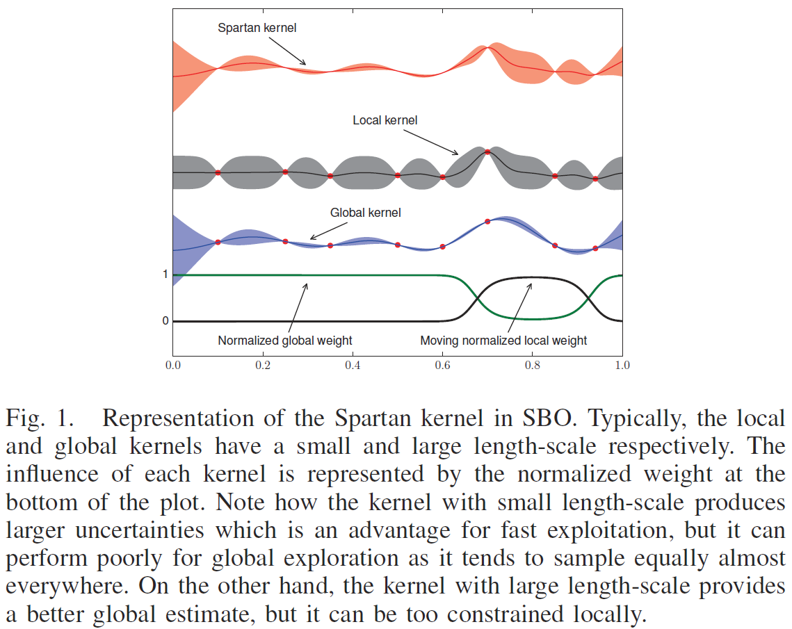
The main contribution of the paper is a new set of adaptive kernels for Gaussian processes that are specifically designed to model functions from nonstationary processes but focused on the local region near the optimum. Thus, the new model maintains the philosophy of global exploration/local exploitation. This idea results in an improved sample efficiency of any Bayesian optimization based on Gaussian processes. We call this new method Spartan Bayesian Optimization (SBO).
II. BAYESIAN OPTIMIZATION WITH GAUSSIAN PROCESSES
The hyperparameters are estimated from data using Markov Chain Monte Carlo (MCMC) resulting in $m$ samples $\Theta = \{\theta_i\}_{i=1}^m$. … The prediction at any point x is a mixture of Gaussians because we use a sampling distribution of $\theta$.
Proposition 1: [18] [1]
Given two kernels kl and ks with large and small length scale hyperparameters respectively, any function f in the RKHS characterized by a kernel kl is also an element of the RKHS characterized by ks.
Thus, using ks instead of kl is safer in terms of guaranteeing convergence.
However, if the small kernel is used everywhere, it might result in unnecessary sampling of smooth areas.
Bayesian optimization is inherently a local stationary process depending on the acquisition function. It has a dual behavior of global exploration and local exploitation. Ideally, both samples and uncertainty estimation end up being distributed unevenly, with many samples and small uncertainty near the local optima and sparse samples and large uncertainty everywhere else.
There have been several attempts to model nonstationarity in Bayesian optimization. Bayesian treed GPs were used in Bayesian optimization combined with an auxiliary local optimizer [19]. An alternative is to project the input space through a warping function to a stationary latent space [20] [2]. Later, Assael et al. [21] [3] built treed GPs where the warping model was used in the leaves. These methods were direct application of regression methods, that is, they model the nonstationary property in a global way. However, as pointed out before, sampling in Bayesian optimization is uneven, thus the global model might end up being inaccurate.
III. SPARTAN BAYESIAN OPTIMIZATION
Our approach to nonstationarity is based on the model presented in Krause & Guestrin [22] [4] where the input space is partitioned in different regions such that the resulting GP is the linear combination of local GPs: $\psi(\bf{x}) = \sum_j \lambda_j(\bf{x})\psi_j(\bf{x})$. Each local GP has its own specific hyperparameters, making the final GP nonstationary even when the local GPs are stationary. (??这里看起来跟 local GP 有点儿相似) In practice, the mixed GP can be obtained by a combined kernel function of the form: $k(\bf{x},\bf{x}'|\theta) = \sum_j \lambda_j(\bf{x}) \lambda_j(\bf{x}'|\theta)$. (??但是 local GP 没有用一个整体 kernel 来推导,而是在每个 local region 分别计算) A related approach of additive GPs was used by Kandasamy et al. [23] [5] for Bayesian optimization of high dimensional functions under the assumption that the actual function is a combination of lower dimensional functions.
 看[4]中的模型。)
For Bayesian optimization, we propose the combination of a local and a global kernels and with multivariate normal distributions as weighting functions. We have called this kernel, the Spartan kernel: (这里的 local kernel 是指上述 [4] 中那种 mixed GP 的 combined kernel function,而不是其中具体的 each local GP。)
Learning the parameters:
As commented in Section II, when new data is available, all the parameters are updated using MCMC.
Therefore, the position of the local kernel $\theta^p$ is moved each iteration to represent the posterior, as can be seen in Figure 2.
Due to the sampling behavior in Bayesian optimization, we found that it intrinsically moves more likely towards the more densely sampled areas in many problems, which corresponds to the location of the function minima.
Furthermore, as we have $m$ MCMC samples, there are $m$ different positions for the local kernel $\Theta_p = \{\theta_i^p\}_{i=1}^m$.
The intuition behind SBO is the same of the sampling strategies in Bayesian optimization: the aim of the model is not to approximate the target function precisely in every point, but to provide information about the location of the minimum. Many optimization problems are difficult due to the fact that the region near the minimum is heteroscedastic, i.e.: it has higher variability than the rest of the space, like the function in Figure 2. In this case, SBO greatly improves the performance of the state of the art in Bayesian optimization.
IV. ACTIVE POLICY SEARCH
V. EVALUATION AND RESULTS
We have selected a variety of benchmarks from the optimization, RL/control and robotics literature.
Although this method allows for any combination of local and global kernels, for the purpose of evaluation, we used the Matérn kernel from equation (3) with ARD for both –local and global– kernels.
Besides, if the target function is stationary, the system might end up learning a similar length-scale for both kernels, thus being equivalent to a single kernel. We can say that standard BO is a special case of SBO where the local and global kernels are the same.
As we will see in the experiments, this is the only drawback of SBO compared to standard BO, as it requires running MCMC in a larger dimensional space, which results in higher computational cost. However, because SBO is more efficient, the extra computational cost can be easily compensated by a reduced number of samples.
- A. Optimization benchmarks
- B. Reinforcement learning experiments
- 1) Walker:
- 2) Mountain Car
- 3) Helicopter hovering
- C. Automatic wing design using CFD simulations
We found that the time differences between the algorithms were mainly driven by the dimensionality and shape of the posterior distribution of the kernel hyperparameters because MCMC was the main bottleneck.