Table of Contents
Gyro Error Models
My Summary (Not finished...)
总体上来讲有两种建模思路。
从控制角度进行仿真,这时重点关注的是 the effect of gyro errors can be compensated for,主要是用 error model 来设计控制器。
从物理角度进行仿真,这里重点关注的是 physical model of the gyro errors,主要是用来研究 gyro 本身的特性,或者进行 high-fidelity 仿真。
从控制的角度考虑
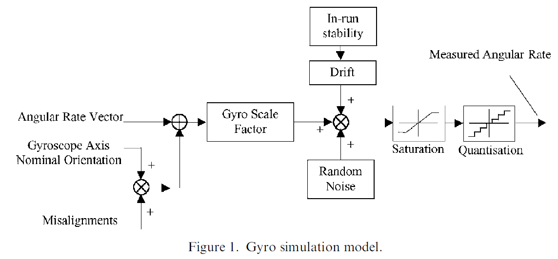
通常可以仿真为 constant bias + rate random walk + white noise (or referred to as angular random walk)。
- 这里的
bias random walk对应的 white noise process 的 $\sigma$ 通常是不直接对应物理意义的,而是一个在设计 EKF 的过程中需要调节的参数 bias random walk又经常被描述为bias drifting,bias instability(注意区分与物理意义上的 bias instability 的不同),没有严格的定义- 这里的
white noise其实包含了后面要说的 gyro errors 的其它物理特性导致的各种 statistical errors。
比如:
- John L. Crassidis, and John L. Junkins, Optimal Estimation of Dynamic Systems, CRC Press, 2011. 中的 Example 3.3, p.167.
- Oliver J Woodman, An introduction to inertial navigation, 2007. link(https://www.cl.cam.ac.uk/techreports/UCAM-CL-TR-696.pdf). 中用 random walk 来建模 bias instability。(这里值得怀疑,待检查)
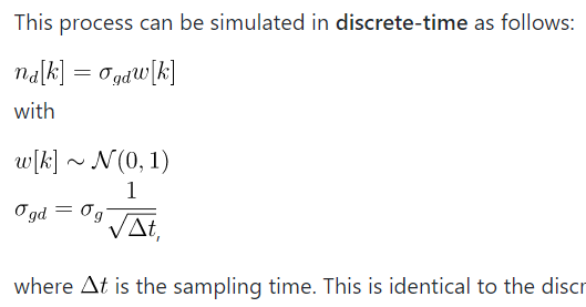
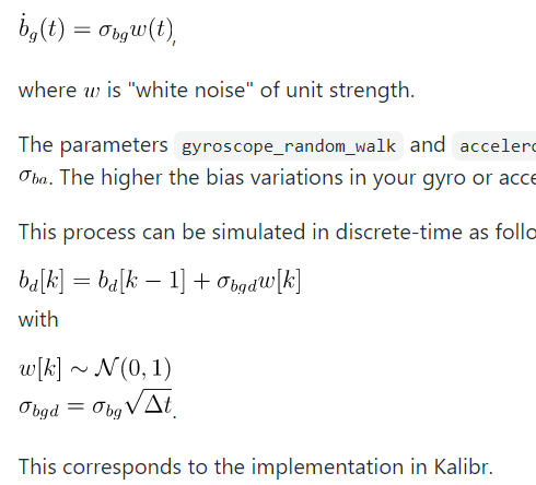
- Kalibr: IMU Noise Model 中详细准确地总结了如何从连续系统推导出离散系统,只建模了random noise和bias drifting。【推荐参考】
按我的理解,这些参数是本质上是应该作为设计 EKF 的一个过程调出来的,因为它们本来就是 controller/estimator 的一部分,但是部分参数可以依据物理元件的参数确定一个范围。
从物理建模的角度考虑
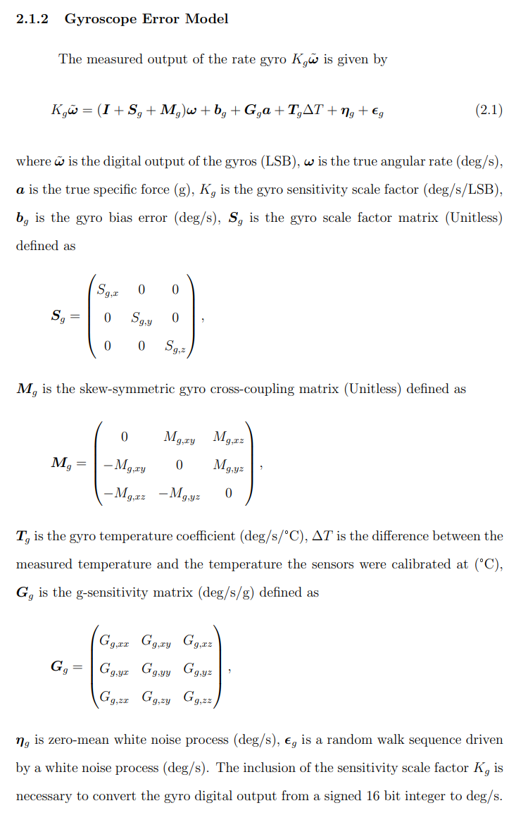
通常会考虑精确的随机过程和依赖于物理参数的误差模型。 元件给出的参数是物理模型的参数。
通常会考虑(See: “IEEE Std 2700-2017 (Revision of IEEE Std 2700-2014) IEEE Standard for Sensor Performance Parameter Definitions”, 2018;只有名义定义和罗列,没有准确的物理意义解释和描述,没有公式,用处不大)
constant biasbias instability:这个是有确定性的定义的,由flicker noise导致的 drifting,建模比较复杂,通常用简单的 first-order Gaussian-Markov model,参考这些文献中的详细描述:- Petko Petkov, and Tsonyo Slavov, “Stochastic Modeling of MEMS Inertial Sensors”, Cybernetics and Information Technologies, vol. 10, 2010, pp. 31–40.
- Elder M. Hemerly, “MEMS IMU stochastic error modelling”, Systems Science & Control Engineering, vol. 5, Jan. 2017, pp. 1–8.
- Vaibhav Saini, S C Rana, and MM Kuber, “Online Estimation of State Space Error Model for MEMS IMU”, Journal of Modelling and Simulation of Systems, vol. 1, 2010, pp. 219–225.
angle random walk:常规理解。rate random walk:常规理解,与从“控制角度”建模时对bias instability的处理类似,仿真成一个离散的 white noise 累加。Rate Ramp Noise:暂时不理解- temperature effect on scale factors
- nonlinearity
QuantizationSaturation- etc.
上述各种参数,用 Allan Variance (AVAR) 工具确定。 AVAR 是一个关于averaging timespan的函数,不是一个值,粗略的思想可以理解为:不同的 noise 在不同时间尺度的平均下会被中和掉,或者反过来讲,在不同时间尺度下不同的 noise 起主导作用。更细致的原理我暂时没有研究。
比如一些参考文献:
- Jay A. Farrell, Felipe O. Silva, Farzana Rahman, and Jan Wendel, “IMU Error State Modeling for State Estimation and Sensor Calibration: A Tutorial”, May 2019. Link(https://escholarship.org/uc/item/1vf7j52p).
- Elder M. Hemerly, “MEMS IMU stochastic error modelling”, Systems Science & Control Engineering, vol. 5, Jan. 2017, pp. 1–8.
- Vaibhav Saini, S C Rana, and MM Kuber, “Online Estimation of State Space Error Model for MEMS IMU”, Journal of Modelling and Simulation of Systems, vol. 1, 2010, pp. 219–225.
- Petko Petkov, and Tsonyo Slavov, “Stochastic Modeling of MEMS Inertial Sensors”, Cybernetics and Information Technologies, vol. 10, 2010, pp. 31–40.
从元器件的参数表确定物理模型的参数
| Names in literatures | Unit | Name on manufacturer's datasheet |
|---|---|---|
| Angular Random Walk | deg/s^(1/2) | Rate noise density; noise density; power spectral density; |
| Bias Stability | deg/s | In Run Bias Stability; Bias Instability; |
| Rate Noise Density | deg/s/Hz^(1/2) | ??? |
| Rate Random Walk |
Random walk (RW) measurement is related to the underlying white noise process' covariance $\sigma^2$ by $RW = \sigma \cdot \sqrt{\delta t}$.
给出 angle random walk (ARW) measurement ($\circ/\sqrt{s}$) 实际上是给明了 bias white noise 的 $\sigma$。 $ARW = \sigma \cdot \sqrt{\delta t}$.
给出 Bias Instability (BI or BS) ($\circ/s$) 和 correlation time 实际上是给出了 bias drifting 的 $\sigma$,应该按照 discrete first-order Gaussian-Markov model 仿真。
Turn-on Bias 是每次开机都不同的固定值,即要被 EKF 估计的值。
如果只是想要一组参数作为仿真数据,查找一些做 statistic noise parameter estimation 的文章,里面通常都会总结几组数据。
Jay A. Farrell, Felipe O. Silva, Farzana Rahman, and Jan Wendel, “IMU Error State Modeling for State Estimation and Sensor Calibration: A Tutorial”, May 2019. Link.
The IMU manufacturer supplies a data sheet characterizing the expected IMU performance, typically in terms of either an Allan Variance (AV) plot or parameters extracted from that plot in accordance with the specification standards [26], [27]. However, it is not immediately clear how to translate information from such data sheets into a suitable state-space model. Such translation methods have been known and used for several decades [28]–[36]. Despite their importance, a clear tutorial exposition of the underlying ideas, issues, and trade-offs is not available in the existing literature. Providing such a tutorial discussion is the purpose of this article. (see [1])
This tutorial discusses the issues and provides an example method by which the navigation system designer can use the information provided by the instrument manufacturer to specify the parameters (e.g., p, nz, Az, Bz, Cz, Qz, and Qη ) for an IMU state-space stochastic error model. Some previous articles have addressed the aforementioned issues [29], [31], [33], [36], [38]–[41]. Our goal herein is to clearly and comprehensively present the background and main ideas in a tutorial fashion, using notation and terminology consistent with instrument specification standards [26], [27]. Examples to clarify issues are included throughout.
Bias in-run stability. The bias in-run stability is the component of the total sensor bias that varies with time in a correlated fashion. This correlated temporal variation is typically modeled as a first-order Gauss-Markov process, i.e., zB(k). … However, the cluster time corresponding to this minimum value is typically not provided by sensor manufacturers, but can be extracted from the ASD plot, if provided; otherwise, the correlation time must be selected and tuned by the designer.
The angle/velocity random walk parameter is the square root of the power spectral density of the sensor inherent white noise, which is denoted by $N$ throughout this paper.
We do not claim that this approach is unique or optimal. It is representative of industrial standard methods.
we have included an extensive discussion of the issues and trade-offs that a designer should consider, including: performance, computational load, observability, and extent of the cluster time τ that is relevant to a given application.
Brief Paper Survey
The Annex-C in the IEEE standard for FOG [2] has defined multiple noise coefficients, inlcuding bias instability coefficient $B$, angular random walk coefficient $N$, rate random walk coefficient $K$, rate ramp coefficient $R$, quantization noise coefÞcient $Q$, etc. Although they are defined for FOG, almost all MEMS gyro error models traced backed to this standard.
Petkov and Slavov [3] presented a detailed methodology to build stochastic discrete-time models of MEMS gyro noise. They used Allan vairance to extract noise coefficient $B$ for bias instability, $N$ for angular random walk, and $K$ for rate random walk. They tested on the ADIS16350 sensor. I cannot reproduce their calculation because Eqs. 4, 6, 9 have some mistakes. However, a log of papers have cited their work and used the $B$, $N$, $K$ values provided in the paper.
Saini et al. [4] also presented an online KF method using EM (Expectation–Maximization) algorithm to estimate MEMS sensor statistic noise parameters. The error model includes $B$, $N$, $K$, $R$. They tested on the IMU from Xsens and summarized parameters obtained via Allan Variance and their online filter.
Hemerly [5] studied ARMA model and KF to online estimate the stochastic model parameters of MEMS gyro. The deficiency with the online methods traces back to the difficulty in estimating $B$ (bias instability) and $K$ (rate random walk) separately under high angular random walk $N$, which is typical of MEMS IMU. He considered mainly $B$, $N$, $K$ in the model and used parameters in [3].
[RECOMMAND THIS ONE] Farrell et al. [1] presented a tutorial about how to build the statistic model for MEMS sensors using datasheet provided by manufactures. They tested on NV IMU-1000 from Nav Technology. A general conclusion to me is that the statistic error model needs tuning even based on manufacturer's specifications (see Sec. IV.F) (their resulting set of parameters can be used directly).
How to read Gyro Datasheets (YouTube)
Robotic Car - How to read Gyro Datasheets (Part 1)
11:45 Different measurements of sensor noise: FFT, PSD, ARW
Robotic Car - How to read Gyro Datasheets (Part 2)
以下内容需要继续整理完善
Collection of some data
Simulations
1. F. Landis Markley, and John L. Crassidis, Fundamentals of Spacecraft Attitude Determination and Control, New York, NY: Springer New York, 2014. link(https://sci-hub.tw/https://link.springer.com/book/10.1007%2F978-1-4939-0802-8).
Example 3.3, pp.167:\beta_0 = 0.1 deg/h \sigma_n = 17e-6 rad \sigma_v = sqrt(10)e-7 rad/s^(1/2) = 3.16e-7 \sigma_u = sqrt(10)e-10 rad/s^(3/2) = 3.16e-10 P_0 = diag[1e-4, 1e-12]
1. Christopher Hide, Terry Moore, and Martin Smith, “Adaptive Kalman Filtering for Low-cost INS/GPS”, The Journal of Navigation, vol. 56, Jan. 2003, pp. 143–152.
The IMU measurements are updated at 100 Hz. The Kalman filter is run in loosely coupled mode with GPS updates at 1 Hz.
Code References
https://github.com/fedecasali/thesis/blob/master/Code/sensormodel.py (forked backup at 01/28/2021)
SeeGyroscope.get_measurementfor handling of different errors.
Seerandom_walkat the end for howbias instabilityis handled.
https://github.com/Aceinna/gnss-ins-sim/blob/master/gnss_ins_sim/sim/imu_model.py (forked backup at 01/28/2021)
Has data of low, middle, high-accuracy MEMS Gyro parameters; model number: AHRS380SA_Datasheet, ADA581016;
seegyro_genandbias_driftatpathgenfor how random walk is handled; aMarkov chainmodel can also be used to replace therandom walkmodel.
这里对 Bias drift (instability) model for accelerometers or gyroscope. 的仿真应该是最正确的,仿真为 first-order Gauss-Markov model。
参考这篇文章的描述:

https://github.com/517030910405/VINS_MONO_TARTANAIR/blob/v1.0/IMU_SIMULATOR/IMU_param.py
Has more gyro parameters here. Based ongnss-ins-sim.
IMU Noise Model in kalibr
What about bias instability? It seems to be different from the bias drifting as described here?
$\sigma_{g}$ corresponds to the values at $\tau=1$.
This is only true since the noise power in most inertial sensors is dominated by “white noise” at a frequency of approximately 1Hz.
$\sigma_{bg}$ is identified as the value of the (fitted) “random walk” diagonal at an integration time of $\tau=3$.
This can be seen immediately when the Allan standard deviation is derived for a “random walk” process [1].
From our experience, for lowest-cost sensors, increasing the noise model parameters by a factor of 10 or more may be necessary.
Obtaining IMU parameterss from datasheet #63
MEMS IMU stochastic error modelling etc
1. Elder M. Hemerly, “MEMS IMU stochastic error modelling”, Systems Science & Control Engineering, vol. 5, Jan. 2017, pp. 1–8.
Experimental works conducted there indicated that MEMS gyroscope stochastic error model is mainly composed of:
(a) bias instability (B), which represents a time varying bias modelled by a first-order Gauss–Markov process;
(b) angular random walk (N), which is an angular error due to white noise in the angular rate
© rate random walk (K), representing a rate error due to white noise in angular acceleration.
In this work, MEMS gyros similar to those investigated in Petkov and Slavov (2010) [see below for this paper] are considered, that is, the most relevant parameters in the stochastic model are B, N and K.
1. Petko Petkov, and Tsonyo Slavov, “Stochastic Modeling of MEMS Inertial Sensors”, Cybernetics and Information Technologies, vol. 10, 2010, pp. 31–40.
MATLAB Documentations
https://www.mathworks.com/help/fusion/ug/introduction-to-simulating-imu-measurements.html#d122e7540
NoiseDensityis the amount of white noise in the sensor measurement. It is sometimes called angle random walk for gyroscopes
BiasInstabilityis the amount of pink or flicker noise in the sensor measurement.
RandomWalkis the amount of Brownian noise in the sensor measurement. It is sometimes called rate random walk for gyroscopes
A Master Thesis
A Technical Report
1. Oliver J Woodman, An introduction to inertial navigation, 2007. link(https://www.cl.cam.ac.uk/techreports/UCAM-CL-TR-696.pdf).
Sections 3 and 4 describe gyroscopes and accelerometers in detail. Both sections contain an overview of the different types of sensors available, as well a description of error sources.
Section 5 introduces Allan Variance, a technique which can be used to detect and measure the noise characteristics of gyroscope and accelerometer signals.
Section 7 describes how simulation can be used to analyse the relative importance of different noise sources. A simple simulator is constructed and verified against the real system developed in Section 6.
3. Gyro
The relative importance of each error source varies across different gyroscopes.
For MEMS gyroscopes angle random walk (noise) errors and uncorrected bias errors either due to uncompensated temperature fluctuations or an error in the initial bias estimation are usually the most important sources of error.
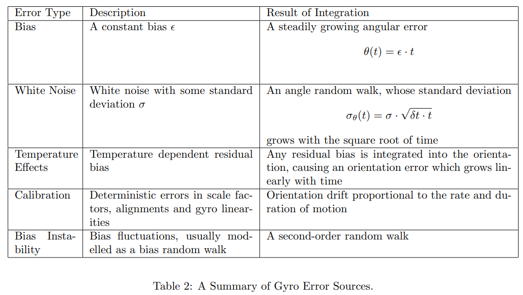
(see Sec 6.1.3) For most MEMS devices white noise and uncorrected bias errors are the main causes of an error in the orientation. White noise causes an angle random walk whose standard deviation grows proportionally to the square root of time. An uncorrected bias causes an error in orientation which grows linearly with time. Quantisation errors also arise in the calculated attitude due to the quantisation of the angular velocity samples and due to the integration scheme used to update $C$.
Constant Bias
The bias of a rate gyro is the average output from the gyroscope when it is not undergoing any rotation (i.e: the offset of the output from the true value)
Thermo-Mechanical White Noise --> Angle Random Walk
The samples obtained from the sensor are perturbed by a white noise sequence, which is simply a sequence of zero-mean uncorrelated random variables. In this case each random variable is identically distributed and has a finite variance $\sigma^2$.
the noise introduces a zero-mean random walk error into the integrated signal, whose standard deviation $\sigma_\theta(t) = \sigma \cdot \sqrt{\delta t \cdot t}$ grows proportionally to the square root of time. $\delta t$ is the time between successive samples. $t = n\cdot\delta t$ is a given timespan.
So, $\delta t$ is fixed and $t$ is varying.
Since we are usually interested in how the noise affects the integrated signal it is common for manufacturers to specify noise using an angle random walk (ARW) measurement $ARW = \sigma_\theta(1)$ with units ${}^\circ/\sqrt{h}$. One gyro having an ARW of $0.2^\circ/\sqrt{h}$ means that after 1 hour the standard deviation of the orientation error will be $0.2^\circ$, after 2 hours it will be $\sqrt{2}\cdot 0.2\approx 0.28^\circ$ and so on.
Other measurements used to specify noise are power spectral density (units $({}^\circ/h)^2/\text{Hz}$) and FFT noise density (units ${}^\circ/h/\sqrt{\text{Hz}})$.
Flicker Noise --> Bias Stability
A bias stability measurement describes how the bias of a device may change over a specified period of time, typically around 100 seconds, in fixed conditions (usually including constant temperature).
Bias stability is usually specified as a 1σ value with units ${}^\circ/h$, or ${}^\circ/s$ for less accurate devices.
In reality bias fluctuations do not really behave as a random walk. If they did then the uncertainty in the bias of a device would grow without bound as the timespan increased. In practice the bias is constrained to be within some range, and therefore the bias random walk model is only a good approximation to the true process for short periods of time.
Temperature Efects
Calibration Errors
The term ‘calibration errors’ refers collectively to errors in the scale factors, alignments, and linearities of the gyros. Such errors tend to produce bias errors that are only observed whilst the device is turning. Such errors lead to the accumulation of additional drift in the integrated signal, the magnitude of which is proportional to the rate and duration of the motions [4]. It is usually possible to measure and correct calibration errors.
Some new IMUs such as the Xsens Mtx apply internal corrections for calibration errors.
5. Signal Noise Analysis: Allan Variance
Allan Variance is a time domain analysis technique originally designed for characterising noise and stability in clock systems. The technique can be applied to any signal to determine the character of the underlying noise processes. The Allan Variance of a signal is a function of averaging time.
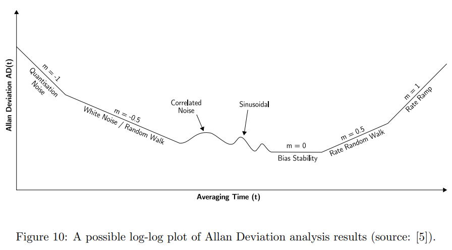
To determine the characteristics of the underlying noise processes, Allan Deviation $AD(t) = \sqrt{AVAR(t)}$ is plotted as a function of $t$ on a log-log scale.
Different types of random process cause slopes with different gradients to appear on the plot
Different processes usually appear in different regions of $t$, allowing their presence to be easily identified:
- White noise appears on the Allan Deviation plot as a slope with gradient $−0.5$. The random walk measurement for this noise (ARW for a rate-gyro, VRW for an accelerometer) is obtained by fitting a straight line through the slope and reading its value at $t = 1$.
- Bias Instability appears on the plot as a flat region around the minimum. The numerical value is
the minimum value on the Allan Deviation curve.
7. Simulation
A fixed bias error $\epsilon$.
An additive Gaussian white noise $N_i$, with a mean of 0 and a standard deviation of $\sigma = \frac{ARW}{\delta t}$, where $ARW = \sigma_{theta}(t=1) = \sigma \sqrt{\delta t \cdot t}$ is the Angle Random Walk measurements.
A random walk sequence $R_i$, where the underlying white noise sequence has a standard deivation of $\sigma = \sqrt{\frac{\delta t}{t}} \cdot BS$, where $t$ is the averaging time at which the bias stability measurement was made. I have strong doubt about this formula!!!
ARW is read from Allan Variance curve by extending slope $-0.5$ line to averaging time 1s.
BS is read from Allan Variance curve as the minimum value, with the averagin timespan $t$ as the corresponding horizontal coordinate.
What is Bias Stability or Bias Instability
https://www.kvhmobileworld.kvh.com/bias-stability-key-parameter-inertial-sensor-performance/
Bias Stability (also known as Bias Instability) can be defined as how much deviation or drift the sensor has from its mean value of the output rate. Essentially, the Bias Stability measurement tells you how stable the bias of a gyro is over a certain specified period of time. Lower Bias Instability is advantageous, as it results in a gyro producing fewer deviations from the mean rate over time.
The bias of a MEMS gyro will wander over time due to flicker noise in the electronics and other effects.
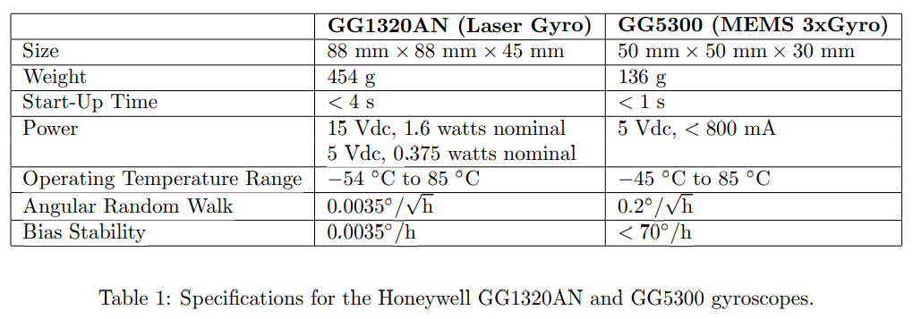
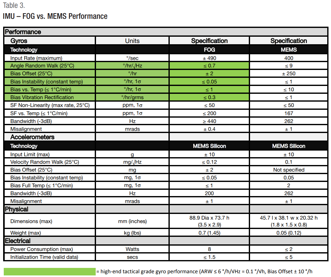
Bias stability is commonly used to determine gyro grades with tactical grades offering bias stability of 0.1°/hr., and navigation grades delivering bias stability of 0.01°/hr.
IMU Specifications (VectorNav Company)
https://www.vectornav.com/resources/imu-specifications
So a single noise standard deviation is insufficient to properly characterize the inherent noisiness of a sensor. While some datasheets will specify that standard deviation at a particular sample rate, the more common measure is noise density which provides the noise divided by the square root of the sampling rate. For example, the noise density for a gyroscope can be represented as °/s/√Hz or °/hr/√Hz. By multiplying the noise density (ND) by the square root of the sampling rate (SR), the noise standard deviation (σ) at that rate can be recovered (σ=ND√SR). Sometimes noise density is specified as a power spectral density, which is simply the noise density squared. In the case of a gyroscope, this yields units of (∘/s)^2/Hz.
The specification for random walk is typically given in units of °/√s or °/√hr for gyroscopes, and m/s/s√ or m/s/√hr for accelerometers. By multiplying the random walk by the square root of time, the standard deviation of the drift due to noise can be recovered.
The bias is a constant offset of the output value from the input value. There are many different types of bias parameters that can be measured, including in-run bias stability, turn-on bias stability or repeatability, and bias over temperature.
The in-run bias stability, or often called the bias instability, is a measure of how the bias will drift during operation over time at a constant temperature. This parameter also represents the best possible accuracy with which a sensor’s bias can be estimated. Due to this, in-run bias stability is generally the most critical specification as it gives a floor to how accurate a bias can be measured.
When a sensor is started up, there is an initial bias present that can fluctuate in value from one turn-on to the next. This change in initial bias at constant conditions (eg. temperature) over the lifetime of the sensor is known as the turn-on bias stability, or is sometimes referred to as bias repeatability.
cannot be calibrated during production due to its varying nature, an aided inertial navigation system (eg. GNSS-aided) can estimate this bias after each startup and account for it in the outputted measurements.
bias temperature sensitivity can be calibrated for after each of these biases are measured over the temperature range. However, this bias can only be measured within the limits of the in-run bias stability.The scale factor error is categorized as one of two equivalent values, either as a parts per million error (ppm), or as an error percentage. Has an example of 0.1% or 1000 ppm. Maybe this is also the value I should use.
| VN-110 | |
| Gyroscope In-Run Bias | < 1°/hr |
| Gyroscope Range | ±490˚/sec |
| IMU Data | 800 Hz |
Guide to Comparing Gyro and IMU Technologies (KVH Industries, Inc.)
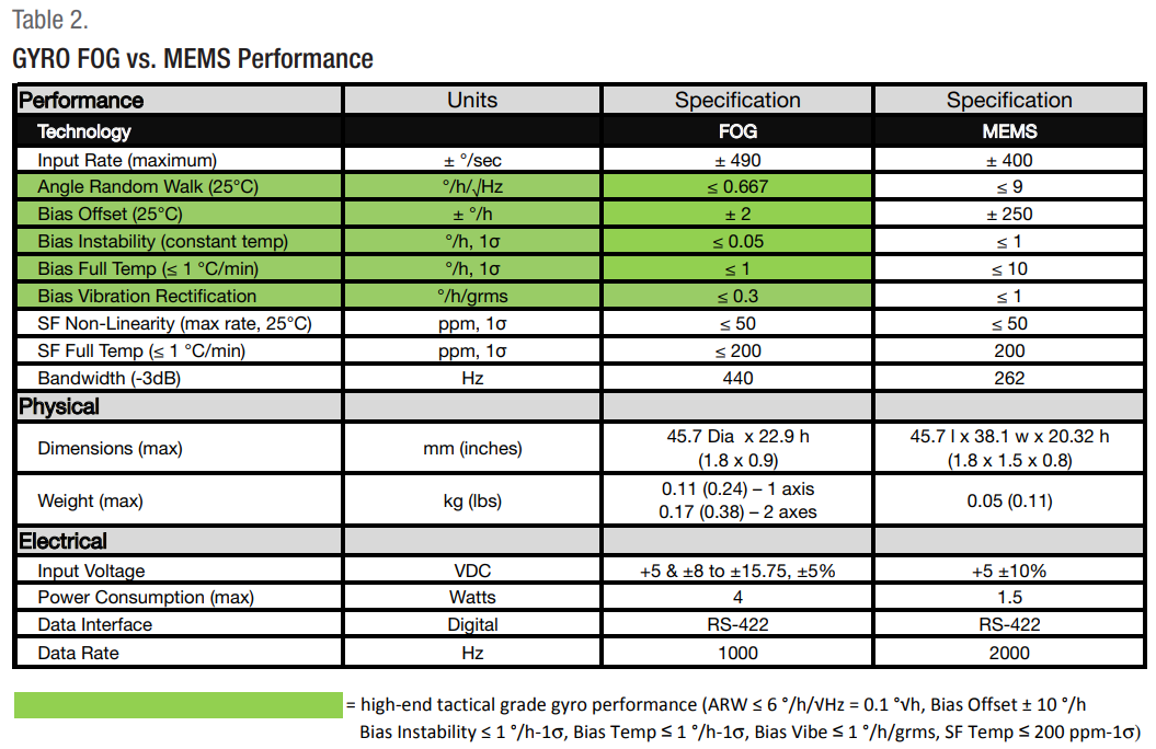
Bias instability is best measured using the Allan Variance (IEEESTD-952) measurement technique and is the fundamental method of deriving
performance specifications for all major gyro types including FOGs, MEMS, and RLGs.
The standard definition of bias instability used by inertial sensor manufacturers is the minimum point on the Allan Variance curve.
Allan Variance is intended to estimate stability due to noise processes, and not that of systematic errors such as temperature, shock, or vibration effects.
While a gyro’s constant bias offset could potentially be calibrated out, bias instability introduces an error that may not be easy to calibrate. Due to bias instability, the longer a gyro operates, the greater its accumulated rate or position error. So, standard attitude determination EKF can estimate the constant bias offset only, but not eliminate bias instability. However, since the EKF is updated at every step with external attitude measurement, can this be treated as a reset of the bias instability? (60% certain it can)
CubeSat gyro
Stellar Gyroscope
1. Samir A. Rawashdeh, James E. Lumpp Jr., James Barrington-Brown, and Massimiliano Pastena, “A Stellar Gyroscope for CubeSat Attitude Determination”, Aug. 2012. link(https://digitalcommons.usu.edu/cgi/viewcontent.cgi?filename=0&article=1078&context=smallsat&type=additional).
Observe the motion of stars in camera’s field of view to infer changes in satellite’s attitude.
Stellar Gyroscope finds relative attitude by tracking stars
In Eclipse, it uses a Stellar Gyroscope to reset the drift of a MEMS attitude propagator.
